- Plotting
- Polynomial
- Random
- Array Creation
- Array Operations
- Matrix Operation
- Args Operations
- Feature Scaling
- Sample ECG Data
- Helper Functions
Plotting
Initialising Plot
int width = 600;
int height = 500;
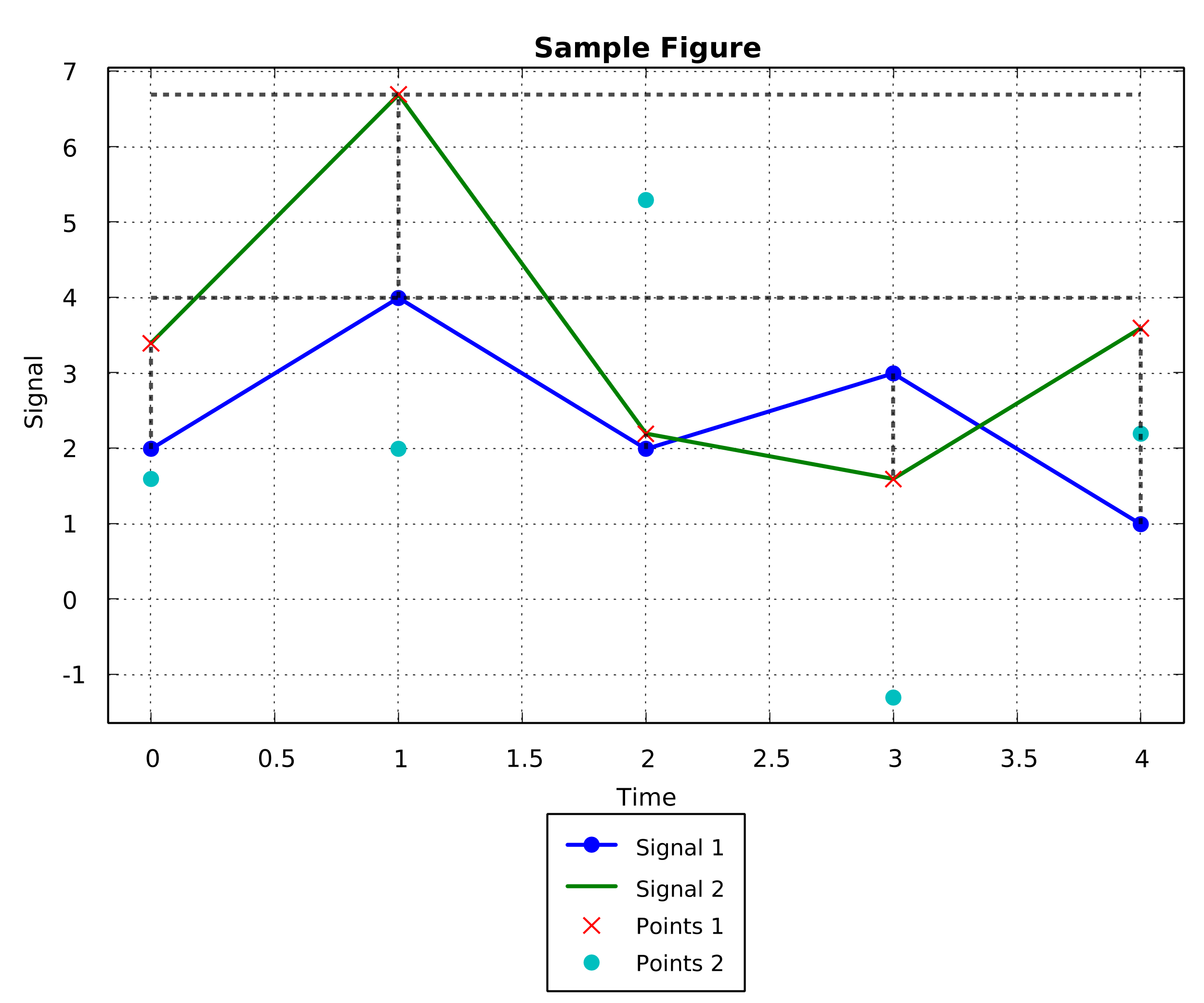
String title = "Sample Figure";
String x_axis = "Time";
String y_axis = "Signal";
Plotting fig = new Plotting(width, height, title, x_axis, y_axis);
fig.initialisePlot();
Add Signals to Plot
double[] signal1 = {2.0, 4.0, 2.0, 3.0, 1.0};
double[] signal2 = {3.4, 6.7, 2.2, 1.6, 3.6};
double[] time = {0.0, 1.0, 2.0, 3.0, 4.0};
fig.addSignal("Signal 1", time, signal1, true);
fig.addSignal("Signal 2", time, signal2, false);
Add Points to Plot
final double[] points1 = {3.4, 6.7, 2.2, 1.6, 3.6};
final double[] points2 = {1.6, 2.0, 5.3, -1.3, 2.2};

fig.addPoints("Points 1", time, points1, 'x');
fig.addPoints("Points 2", time, points2);
Add Horizontal/Vertical Line
// For vertical lines
double[][] verLines = {{0.0, 2.0, 3.4},
                        {1.0, 4.0, 6.7},
                        {2.0, 2.0, 2.2},
                        {3.0, 3.0, 1.6},
                        {4.0, 1.0, 3.6}};

for (int i=0; i<=verLines.length-1; i++) {
    fig.vline(verLines[i][0], verLines[i][1], verLines[i][2]);
}

// For horizontal lines
fig.hline(0.0, 4.0, 4.0);
fig.hline(0.0, 4.0, 6.7);
Displaying & Saving the Plot
String outputFileName = "signal.png";
// To plot on a window
fig.plot();
// To save as an image
fig.saveAsPng(outputFileName);
Fitting a Polynomial Function
Code
double[] x = {0.0, 1.0, 2.0, 3.0,  4.0,  5.0};
double[] y = {0.0, 0.8, 0.9, 0.1, -0.8, -1.0};
double[] out = Polynomial.polyfit(x, y, 3);
Output
[0.087, -0.8135, 1.6931, -0.0397] ⇨ 0.087x3 - 0.8135x2 + 1.6931x - 0.0387
Polynomial Function Evaluation
Code
double[] coeffs = {3.0, 0.0, 1.0}; // 3x2 + 1
double x_val = 5.0;
double out_val = Polynomial.polyval(coeffs, x_val);
double[] x_arr = {5.0, 3.2, 1.2};
double[] out_arr = Polynomial.polyval(coeffs, x_arr);
Output
out_val ⇨ 76.0
out_arr ⇨ [76.0  , 31.72,  5.32]
Derivative of a Polynomial Function
Code
double[] coeffs = {6, 3, 1, 1}; // 6x3 + 3x2 + x + 1
int m2 = 2; //Order of derivative
double[] out2 = Polynomial.polyder(coeffs, m2);
Output
[18, 6, 1] ⇨ 18x2 + 6x + 1
Anti-Derivative of a Polynomial Function
Code
double[] coeffs = {140, 390, 80, 110}; // 140x3 + 390x2 + 80x + 110
double[] constants = {17, 34};
int order = 2; //Order of anti-derivative
double[] out2 = Polynomial.polyint(coeffs, m2, constants);
Output
[7.0, 32.5, 13.33, 55, 17, 34] ⇨ 7x5 + 32.5x4 + 13.33x3 + 55x2 + 17x + 34
Generate a Random Sample
Code
Random r1 = new Random();
r1.setSeed(42); //OPTIONAL
double xNorm = r1.randomNormalSample(); //Generates a Sample from a Normal Distribution
double xDouble = r1.randomDoubleSample(); //Generates a Sample between 0.0 and 1.0
int xInt = randomIntSample(5); //Generates a Sample between 0 and 5
Generate a Random 1D Array
Code
Random r1 = new Random(110); //Set seed to 110
double[] xNorm = r1.randomNormal1D(new int[]{5}); //Generates an array of 5 samples from a Normal Distribution
double[] xDouble = r1.randomDouble1D(new int[]{5}); //Generates an array of 5 samples between 0.0 and 1.0
int[] xInt = randomInt1D(new int[]{5}, 2, 10); //Generates an array of 5 samples between 2 and 10
Generate a Random 2D Array
Code
Random r1 = new Random(110); //Set seed to 110
double[][] xNorm = r1.randomNormal2D(new int[]{5,5}); //Generates a 2D matrix of 5x5 samples from a Normal Distribution
double[][] xDouble = r1.randomDouble2D(new int[]{5,5}); //Generates a 2D matrix of 5x5 samples between 0.0 and 1.0
int[][] xInt = randomInt2D(new int[]{5,5}, 2, 10); //Generates a 2D matrix of 5x5 samples between 2 and 10
Generate a Random 3D Array
Code
Random r1 = new Random();
double[][][] xNorm = r1.randomNormal3D(new int[]{5,5,5}); //Generates a 3D matrix of 5x5x5 samples from a Normal Distribution
double[][][] xDouble = r1.randomDouble3D(new int[]{5,5,5}); //Generates a 3D matrix of 5x5x5 samples between 0.0 and 1.0
int[][][] xInt = randomInt3D(new int[]{5,5,5}, 2, 10); //Generates a 3D matrix of 5x5x5 samples between 2 and 10
Linspace
Code
int start = 2;
int stop = 3;
int samples = 5;
boolean includeEnd = true;
double[] out1 = UtilMethods.linspace(start, stop, samples, includeEnd);
Output
[2.0, 2.25, 2.50, 2.75, 3.0]
Linspace with Repeated Elements
Code
int start = 2;
int stop = 3;
int samples = 5;
int repeats = 2;
double[] out = UtilMethods.linspace(start, stop, samples, repeats);
Output
[2.0, 2.25, 2.50, 2.75, 3.0, 2.0, 2.25, 2.50, 2.75, 3.0]
Arange
Code
double start = 3.0; //Can be int
double stop = 9.0; //Can be int
double step = 0.5; //Can be int
double[] out = UtilMethods.arange(start, stop, step);
Output
[3.0, 3.5, 4.0, 4.5, 5.0, 5.5, 6.0, 6.5, 7.0, 7.5, 8.0, 8.5]
Reverse Array
Code
double[] arr = {1.0, 2.0, 3.0, 4.0, 5.0, 6.0}; //Can be int[]
double[] out = UtilMethods.reverse(arr);
Output
[6.0, 5.0, 4.0, 3.0, 2.0, 1.0]
Concatenate Arrays
Code
double[] arr1 = {1.0, 2.0}; //Can be int[]
double[] arr2 = {3.0, 4.0, 5.0, 6.0}; //Can be int[]

double[] out = UtilMethods.concatenateArray(arr1, arr2);
Output
[1.0, 2.0, 3.0, 4.0, 5.0, 6.0]
Split Arrays by Index
Code
double[] signal = {1.0, 2.0, 3.0, 4.0, 5.0, 6.0}; //Can be int[]
int start = 2;
int stop = 5;
double[] out = UtilMethods.splitByIndex(signal, start, stop);
Output
[3.0, 4.0, 5.0]
Padding an Array
Code
double[] signal = {2, 8, 0, 4, 1, 9, 9, 0};
double[] reflect = UtilMethods.padSignal(signal, "reflect");
double[] constant = UtilMethods.padSignal(signal, "constant");
double[] nearest = UtilMethods.padSignal(signal, "nearest");
double[] mirror = UtilMethods.padSignal(signal, "mirror");
double[] wrap = UtilMethods.padSignal(signal, "wrap");
Output
reflect: [0, 9, 9, 1, 4, 0, 8, 2, 2, 8, 0, 4, 1, 9, 9, 0, 0, 9, 9, 1, 4, 0, 8, 2]
constant: [0, 0, 0, 0, 0, 0, 0, 0, 2, 8, 0, 4, 1, 9, 9, 0, 0, 0, 0, 0, 0, 0, 0, 0]
nearest: [2, 2, 2, 2, 2, 2, 2, 2, 2, 8, 0, 4, 1, 9, 9, 0, 0, 0, 0, 0, 0, 0, 0, 0]
mirror: [9, 0, 9, 9, 1, 4, 0, 8, 2, 8, 0, 4, 1, 9, 9, 0, 9, 9, 1, 4, 0, 8, 2, 8]
wrap: [2, 8, 0, 4, 1, 9, 9, 0, 2, 8, 0, 4, 1, 9, 9, 0, 2, 8, 0, 4, 1, 9, 9, 0]
Nth Discrete Difference
Code
double[] seq = {1, 2, 3, 4, 6, -4};
double[] out = UtilMethods.diff(seq);
Output
[1, 1, 1, 2, -10]
Unwrap
Code
double[] seq = {0.0 , 0.78539816, 1.57079633, 5.49778714, 6.28318531};
double[] out = UtilMethods.unwrap(seq);
Output
[0.0, 0.785, 1.571, -0.785, 0.0]
Absolute Value of Array
Code
double[] a = {1.22, -3.41, -0.22, 5.44, -9.28};
double[] out = UtilMethods.absoluteArray(a);
Output
[1.22, 3.41, 0.22, 5.44, 9.28]
Scalar Arithmetic on Array
Code
double[] signal = {1.23, 6.54, 4.56, 9.04, 2.88};
double[] addArr = UtilMethods.scalarArithmetic(signal, 1.02, "add");
double[] subArr = UtilMethods.scalarArithmetic(signal, 1.02, "sub");
double[] mulArr = UtilMethods.scalarArithmetic(signal, 1.02, "mul");
double[] divArr = UtilMethods.scalarArithmetic(signal, 1.02, "div");
Output
addArr: [2.25,  7.56,  5.58, 10.06,  3.9]
subArr: [0.21, 5.52, 3.54, 8.02, 1.86]
mulArr: [1.2546, 6.6708, 4.6512, 9.2208, 2.9376]
divArr: [1.2059, 6.4118, 4.4706, 8.8627, 2.8235]
Trigonometric Arithmetic on Array
Code
double[] arr1 = {1.23, 6.54, 4.56, 9.04, 2.88};
double[] sinArr = UtilMethods.trigonometricArithmetic(arr1, "sin");
double[] cosArr = UtilMethods.trigonometricArithmetic(arr1, "cos");
double[] tanArr = UtilMethods.trigonometricArithmetic(arr1, "tan");

double[] arr2 = {-0.92, -0.38, 0.25, 0.55, 0.98};
double[] asinArr = UtilMethods.trigonometricArithmetic(arr2, "asin");
double[] acosArr = UtilMethods.trigonometricArithmetic(arr2, "acos");
double[] atanArr = UtilMethods.trigonometricArithmetic(arr2, "atan");
Output
sinArr: [0.9425 ,  0.2540  , -0.9884,  0.3754,  0.2586]
cosArr: [0.3342,  0.9672, -0.1518, -0.9269 , -0.9660]
tanArr: [2.8198,  0.2626,  6.5113, -0.4050, -0.2677]

asinArr: [-1.1681, -0.3898,  0.2527,  0.5824,  1.3705]
acosArr: [2.7389, 1.9606, 1.3181, 0.9884, 0.2003]
atanArr: [-0.7438, -0.3631,  0.2450,  0.5028,  0.7753]
Sinc Value of Array Elements
Code
double[] x_arr = {0.1, 0.2, 0.3, 0.4, 0.5, 0.6, 0.7, 0.8, 0.9};
double[] out_arr = UtilMethods.sinc(x_arr);
Output
[0.9836, 0.9355, 0.8584, 0.7568, 0.6366, 0.5046, 0.3679, 0.2339, 0.1093]
Pseudo-inverse of Matrix
Code
double[][] matrix = {{1.0, 2.0, 3.0}, {4.0, 5.0, 6.0}, {7.0, 8.0, 9.0}};
double[][] out = UtilMethods.pseudoInverse(matrix);
Output

Matrix Multiplication
Code
double[][] m1 = {{1.0, 2.0, 3.0}, {4.0, 5.0, 6.0}, {7.0, 8.0, 9.0}};
double[][] m2 = {{1.0, 2.0, 3.0}, {4.0, 5.0, 6.0}, {7.0, 8.0, 9.0}};
double[][] out = UtilMethods.matrixMultiply(m1, m2);
Output

Matrix Transpose
Code
double[][] matrix = {{1.0, 2.0, 3.0}, {4.0, 5.0, 6.0}, {7.0, 8.0, 9.0}};
double[][] out = UtilMethods.transpose(matrix);
Output

Absolute Value of Matrix
Code
double[][] m1 = {{1.22, -3.41, -0.22}, {-0.89, 1.6, 7.65}};
double[][] out = UtilMethods.absoluteArray(m1);
Output

2D Array Operations
Addition
Subtraction
double[][] m1 = {{1.0, 2.0, 3.0}, {4.0, 5.0, 6.0}, {7.0, 8.0, 9.0}};
double[][] m2 = {{1.0, 2.0, 3.0}, {4.0, 5.0, 6.0}, {7.0, 8.0, 9.0}};
double[][] out = {{2.0, 4.0, 6.0}, {8.0, 10.0, 12.0}, {14.0, 16.0, 18.0}};
double[][] m1 = {{1.0, 2.0, 3.0}, {4.0, 5.0, 6.0}, {7.0, 8.0, 9.0}};
double[][] m2 = {{1.0, 2.0, 3.0}, {4.0, 5.0, 6.0}, {7.0, 8.0, 9.0}};
double[][] out = {{0.0, 0.0, 0.0}, {0.0, 0.0, 0.0}, {0.0, 0.0, 0.0}};


Element-by-Element Operations
Addition
Subtraction
double[][] m1 = {{1.0, 2.0}, {2.0, 0.5}, {3.0, 4.0}};
double[][] m2 = {{1.0, 2.0}, {2.0, 0.5}, {3.0, 4.0}};
RealMatrix out = UtilMethods.ebeAdd(MatrixUtils.createRealMatrix(m1), MatrixUtils.createRealMatrix(m2));
double[][] m1 = {{1.0, 2.0}, {2.0, 0.5}, {3.0, 4.0}};
double[][] m2 = {{1.0, 2.0}, {2.0, 0.5}, {3.0, 4.0}};
RealMatrix out = UtilMethods.ebeSubtract(MatrixUtils.createRealMatrix(m1), MatrixUtils.createRealMatrix(m2));

Multiplication
Division
double[][] m1 = {{1.0, 2.0}, {2.0, 0.5}, {3.0, 4.0}};
double[][] m2 = {{1.0, 2.0}, {2.0, 0.5}, {3.0, 4.0}};
RealMatrix out = UtilMethods.ebeMultiply(MatrixUtils.createRealMatrix(m1), MatrixUtils.createRealMatrix(m2));
double[][] m1 = {{1.0, 2.0}, {2.0, 0.5}, {3.0, 4.0}};
double[][] m2 = {{1.0, 2.0}, {2.0, 0.5}, {3.0, 4.0}};
RealMatrix out = UtilMethods.ebeDivide(MatrixUtils.createRealMatrix(m1), MatrixUtils.createRealMatrix(m2));


Row-wise Operations
Addition
Subtraction
double[][] m1 = {{1.0, 2.0}, {2.0, 0.5}, {3.0, 4.0}};
double[][] m2_row = {{0.5, 1.0}};
RealMatrix out = UtilMethods.ebeAdd(MatrixUtils.createRealMatrix(m1), MatrixUtils.createRealMatrix(m2_row), "row");
double[][] m1 = {{1.0, 2.0}, {2.0, 0.5}, {3.0, 4.0}};
double[][] m2_row = {{0.5, 1.0}};
RealMatrix out = UtilMethods.ebeSubtract(MatrixUtils.createRealMatrix(m1), MatrixUtils.createRealMatrix(m2_row), "row");


Multiplication
Division
double[][] m1 = {{1.0, 2.0}, {2.0, 0.5}, {3.0, 4.0}};
double[][] m2_row = {{0.5, 1.0}};
RealMatrix out = UtilMethods.ebeMultiply(MatrixUtils.createRealMatrix(m1), MatrixUtils.createRealMatrix(m2_row), "row");
double[][] m1 = {{1.0, 2.0}, {2.0, 0.5}, {3.0, 4.0}};
double[][] m2_row = {{0.5, 1.0}};
RealMatrix out = UtilMethods.ebeDivide(MatrixUtils.createRealMatrix(m1), MatrixUtils.createRealMatrix(m2_row), "row");


Column-wise Operations
Addition
Subtraction
double[][] m1 = {{1.0, 2.0}, {2.0, 0.5}, {3.0, 4.0}};
double[][] m2_col = {{0.5}, {1.0}, {2.0}};
RealMatrix out = UtilMethods.ebeAdd(MatrixUtils.createRealMatrix(m1), MatrixUtils.createRealMatrix(m2_col), "column");
double[][] m1 = {{1.0, 2.0}, {2.0, 0.5}, {3.0, 4.0}};
double[][] m2_col = {{0.5}, {1.0}, {2.0}};
RealMatrix out = UtilMethods.ebeSubtract(MatrixUtils.createRealMatrix(m1), MatrixUtils.createRealMatrix(m2_col), "column");


Multiplication
Division
double[][] m1 = {{1.0, 2.0}, {2.0, 0.5}, {3.0, 4.0}};
double[][] m2_col = {{0.5}, {1.0}, {2.0}};
RealMatrix out = UtilMethods.ebeMultiply(MatrixUtils.createRealMatrix(m1), MatrixUtils.createRealMatrix(m2_col), "column");
double[][] m1 = {{1.0, 2.0}, {2.0, 0.5}, {3.0, 4.0}};
double[][] m2_col = {{0.5}, {1.0}, {2.0}};
RealMatrix out = UtilMethods.ebeDivide(MatrixUtils.createRealMatrix(m1), MatrixUtils.createRealMatrix(m2_col), "column");


Argument of the Minimum
Code
double[][] matrix = {{1.0, 2.0, 3.0}, {4.0, 5.0, 6.0}, {7.0, 8.0, 9.0}};
double[][] out = UtilMethods.pseudoInverse(matrix);
Output
       min1 = 0
       min2 = 6
Argument of the Maximum
Code
double[] arr = {1, 2, 5, 3, 4, 6, 1, 6};
int max1 = UtilMethods.argmax(arr, false); //Returns the last occurrence index if more than 1 max value
int max2 = UtilMethods.argmax(arr, true); //Returns the first occurrence index if more than 1 max value
Output
       max1 = 5
       max2 = 7
Indices to sort array
Code
double[] test1 = {1.23, 4.55, -1.33, 2.45, 6.78, 1.29};
int[] sortedIndices = UtilMethods.argsort(test1, true); //In ascending order
Output
[2, 0, 5, 3, 1, 4]
Rescale
Code
double[] arr1 = {12, 14, 15, 15, 16};
double[] out1 = UtilMethods.rescale(arr1, 10, 20);
Output
[10, 15, 17.5, 17.5, 20]
Standardize
Code
double[] arr1 = {12, 14, 15, 15, 16};
double[] out1 = UtilMethods.standardize(arr1);
Output
[0, 0.5, 0.75, 0.75, 1]
Normalize
Code
double[] arr1 = {12, 14, 15, 15, 16};
double[] out1 = UtilMethods.normalize(arr1);
Output
[-1.583, -0.264, 0.396, 0.396, 1.055]
Zero Center
Code
double[] arr1 = {12, 14, 15, 15, 16};
double[] out1 = UtilMethods.zeroCenter(arr1);
Output
[-2.4, -0.4, 0.6, 0.6, 1.6]
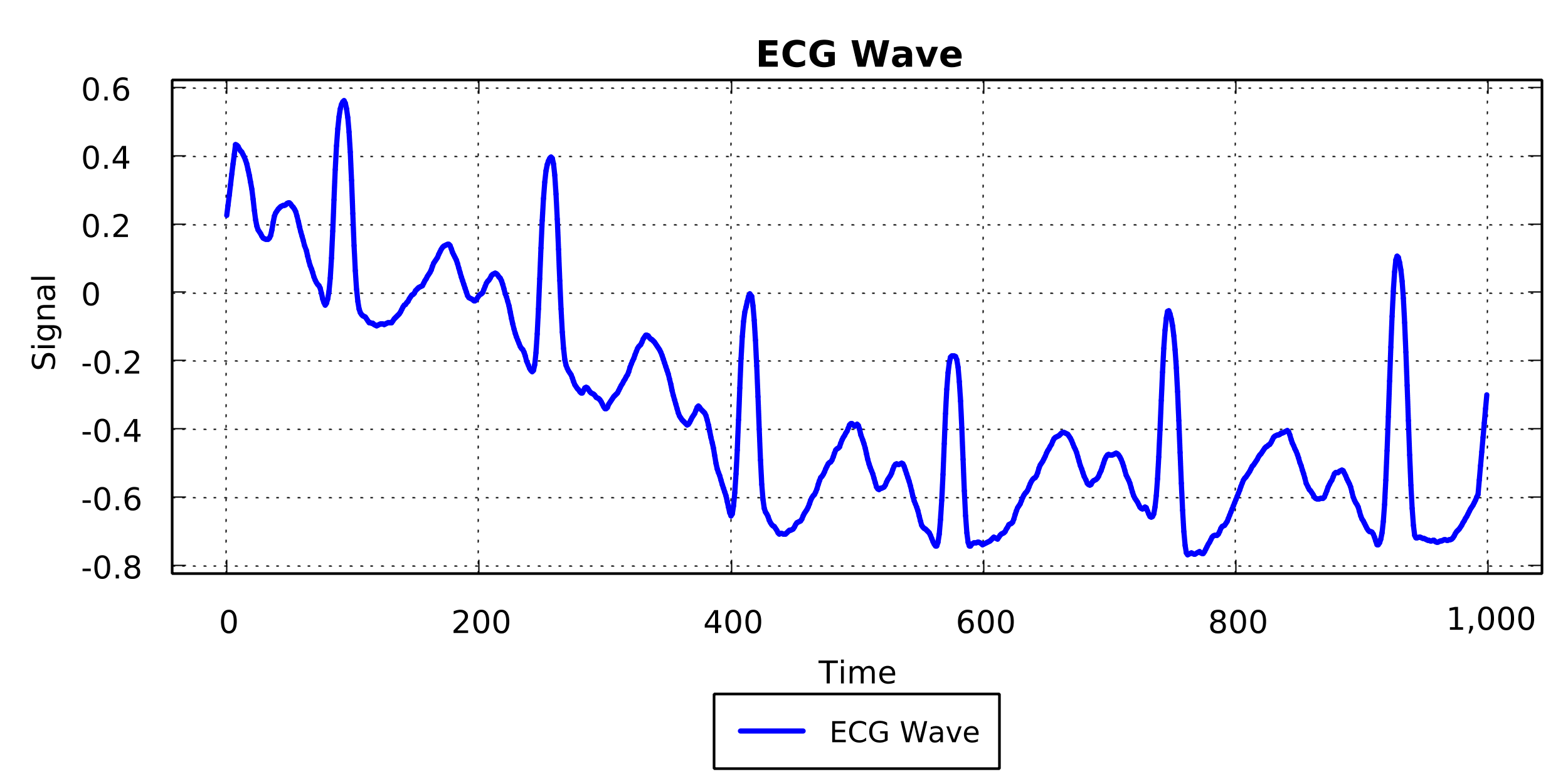
ECG Signal
Getting Raw Data
double[] rawData = UtilMethods.electrocardiogram();
Simple Processing
double[] data = UtilMethods.splitByIndex(rawData, 3200, 4200);
Smooth sObj = new Smooth(data, 15, "rectangular");
double[] ecgSignal = sObj.smoothSignal("same");
double[] time = UtilMethods.arange(0, (double)ecgSignal.length, 1);
Saving the Plot
Plotting fig = new Plotting(600, 300, "ECG Wave", "Time", "Signal");
fig.initialise_plot();
fig.add_signal("ECG Wave", time, ecgSignal, false);
fig.save_as_png("ecg.png");
Rounding to nth Decimal
Code
double val = 123.45667;
double out = UtilMethods.round(val, 1);
Output
123.5
Rounding to nth Decimal for double[] array
Code
double[] arr = {7.40241449, -14.34767505,  12.88704602,   5.81646305};
double[] out = UtilMethods.round(arr, 1);
Output
[7.4, -14.3, 12.9, 5.8]
Modulus Operation (Python)
Code
double divisor = -2;
double dividend = 4;
double out = UtilMethods.modulo(divisor, dividend);
Output
2
Convert Integer ArrayList to Primitive int[]
Code
ArrayList< Integer > integers = new ArrayList< Integer >(Arrays.asList(1, 2, 3, 4, 5));double[] test2 = {1.23310, 1.23320};
int[] out1 = UtilMethods.convertToPrimitiveInt(integers)
Convert Integer ArrayList to Primitive double[]
Code
ArrayList< Double > numbers = new ArrayList< Double >(Arrays.asList(1.1, 2.22, 3.3, 4.4, 5.55));
double[] out2 = UtilMethods.convertToPrimitiveDouble(numbers);
Chebyshev Evaluation
Code
double[] arr = {1000.0, 2.0, 3.4, 17.0, 50.0};
double[] x_arr = {1.0, 2.0, 3.0, 4.0, 5.0};
double[] out_arr = UtilMethods.chebyEval(x_arr, arr);
Output
[-470.2, 1047.4, 23580.4, 97134.8, 263716.6]
Vector to Matrix Transform
Hankel
Toeplitz
double[] c = {1, 2, 3, 4};
double[] r = {4, 7, 7, 8, 9};
double[][] output = UtilMethods.hankel(c, r);
double[] c = {1,2,3,4};
double[][] output = UtilMethods.toeplitz(c);

